All projectsPrototype · 03
CHIP: Cloud-Honest Image Pipeline
A solo build for the IBM BoB Hackathon that turns one sentence into a Sentinel-2 image chip, scoring cloud over the area actually asked about and applying the reflectance offset most scripts miss. Two scenes show why.
- Sep 2026
- Solo hackathon entrant
- 1
- Data engineering
- Python · FastAPI · rasterio · NumPy · STAC · Sentinel-2
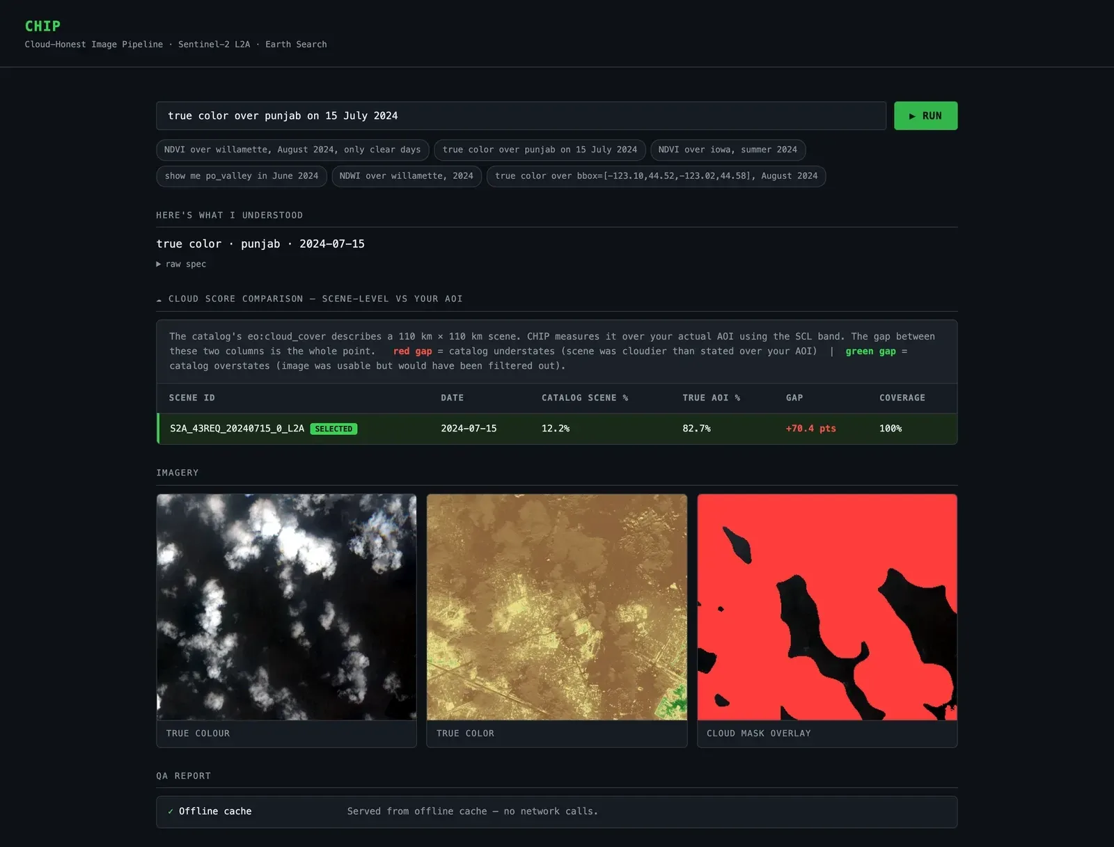
The web page in offline mode for the Punjab scene: the catalogue says 12.2% cloud, the area is 82.7%. Contains modified Copernicus Sentinel data 2024.
Problem & constraints
A common way to pick Sentinel-2 scenes is to filter on eo:cloud_cover. That number describes a whole tile, about 110 km across, while the two example areas below are each about 7–8 km wide. So the filter can answer a different question from the one being asked, and the examples show it failing in both directions without raising an error.
Two real scenes show it. Over farmland near Ludhiana, Punjab, on 15 July 2024, the catalogue says 12.2% cloud: the scene passes a typical < 20% filter, but the area of interest is 82.7% cloud. Over the Willamette Valley on 2 August 2024, the catalogue says 47.4%: the scene is filtered out, but the area is 1.9% cloud.
A second silent error compounds it. Since processing baseline 04.00 (January 2022), Sentinel-2 L2A reflectance is (DN − 1000) / 10000, not DN / 10000. On the clear Willamette scene, leaving out the offset gives a mean NDVI of 0.299 instead of 0.497. The result is about 40% low and still looks plausible.
CHIP was my entry to the IBM BoB Hackathon (AI After Hours, 17 September 2026), where every product had to be built with IBM's Bob coding agent in under two hours. On its "fix something broken" track I planned a 90-minute build, and CHIP had to make both errors visible to someone who only types a sentence.
Remote-sensing analysts who pull one area of interest at a time from a STAC catalogue.
- Under two hours to build, with IBM's Bob coding agent (IBM BoB Hackathon, track "Fix It"); I planned for 90 minutes.
- Public data only: Sentinel-2 L2A Cloud-Optimized GeoTIFFs on AWS, found through Earth Search.
- It had to run with no API keys, and offline for the demo.
- Small dependency set: rasterio, numpy, Pillow, requests, FastAPI. No database, no front-end build.
My role
A solo entry. I framed the problem, measured the two example scenes, prepared the demo data and wrote the build spec and tickets. IBM's Bob coding agent, which the hackathon required every entry to use, wrote the application code from that spec, ticket by ticket.
Architecture
One sentence goes in; a chip, its statistics and a QA report come out. The same pipeline backs a CLI, a FastAPI JSON API and a single-file web page.
flowchart TB
  S["Sentence"] --> P["parse: rules first, optional LLM fallback"]
  P --> Q["QuerySpec: area, dates, product, cloud limit"]
  Q --> ST["STAC search on Earth Search, no cloud filter"]
  ST --> R["Rank up to 8 candidates by cloud over the area (SCL band)"]
  R --> B["Windowed reads of the red, green, blue and NIR bands"]
  B --> O["Apply the reflectance offset; render true colour, NDVI or NDWI"]
  O --> C["Five QA checks"]
C --> OUT["CLI, JSON API, web page"]- Search asks Earth Search for every scene in the date range, with no cloud filter, so a good scene can't be thrown away before it is looked at.
- Ranking reads only the Scene Classification Layer (SCL) window over the area of interest for each candidate, counts cloud, cloud-shadow and cirrus pixels, and picks the clearest. Every loser stays in the comparison table, next to its catalogue number.
- Products read just the window of each band from the Cloud-Optimized GeoTIFFs, apply the offset for the scene's processing baseline and write a PNG (and a GeoTIFF).
- QA reports the offset's effect, catalogue vs area cloud disagreement, nodata handling, the output CRS and the share of valid pixels.
- Offline mode serves the two example scenes from cached STAC items and pre-rendered images, so the demo makes no network calls.
Diagram description
Flowchart, top to bottom: a sentence is parsed (rules first, an optional LLM fallback) into a QuerySpec with area, dates, product and cloud limit. A STAC search on Earth Search runs with no cloud filter. Up to eight candidate scenes are ranked by cloud measured over the area with the SCL band. The winner’s red, green, blue and near-infrared bands are read as windows, the reflectance offset is applied and a true-colour, NDVI or NDWI image is rendered. Five QA checks run, and the result goes to the CLI, the JSON API and the web page.
Key decisions
Measure cloud over the area, not the tile
The catalogue value is a tile-wide average, and the example scenes are wrong by 70 points in one direction and 46 in the other.
- Search without a cloud filter, then read the SCL band over the area of interest for up to eight candidates and rank them by that number. Show both numbers side by side.
- Each candidate costs an extra windowed read, so ranking is capped at eight scenes. SCL is itself a classifier and has its own errors.
Alternatives considered (2)
- Keep the usual `eo:cloud_cover` filter — It is the bug: it admits the cloudy Punjab scene and rejects the clear Willamette one.
- Run a separate cloud-detection model on the pixels — Out of scope for 90 minutes and a laptop. SCL is already computed by ESA for every L2A scene.
Rules first, language model optional
The input is a sentence, but the demo had to work with no API key and no network.
- A deterministic regex parser handles the supported phrasings (named areas, a bounding box, dates, "only clear days"). An optional IBM watsonx Granite call is tried only when a key is set, and any error falls back to the rules.
- The grammar is narrow: four named areas plus explicit bounding boxes, and a fixed set of date phrases.
Alternatives considered (1)
- Parse every sentence with an LLM — Needs a key and a network, adds latency, and makes the parse harder to test. The acceptance tests run with the LLM disabled.
Fix the offset and say so
Missing the processing-baseline offset changes the answer without breaking anything.
- Apply the offset whenever the scene’s baseline needs it, and add a QA check that reports what NDVI would have been without it.
- The QA report is longer, and the counterfactual costs a second NDVI computation.
Alternatives considered (1)
- Correct it silently — The user would never learn that their other scripts are wrong, which was the point of the entry.
Outcomes & evidence
Catalogue 12.23% vs area 82.65% (S2A_43REQ_20240715_0_L2A)
On the Punjab example scene, the catalogue reports 12.2% cloud, but the area of interest is 82.7% cloud.
One of two example scenes (n = 2), not a general error rate. Cloud = SCL classes 3, 8, 9 and 10 over the area’s window; valid pixels 100%. Re-measured on 24 Sep 2026 (UTC) from the public COGs with the repository’s acceptance tests and `aoi_cloud_fraction`; the values match the ones recorded in the repository.
Source for this outcome (opens in a new tab)Catalogue 47.44% vs area 1.89% (S2B_10TDQ_20240802_0_L2A)
On the Willamette example scene, the catalogue reports 47.4% cloud, but the area of interest is 1.9% cloud.
The second of the two example scenes (n = 2). Same method and re-measurement as above.
Source for this outcome (opens in a new tab)Mean NDVI 0.2989 without the offset vs 0.4974 with it
Leaving out the reflectance offset lowers mean NDVI on the clear Willamette scene by about 40%.
Mean NDVI over the Willamette area window, computed with and without the baseline offset (`test_reflectance_offset_changes_ndvi_materially`). One scene; re-measured on 24 Sep 2026 (UTC).
Source for this outcome (opens in a new tab)All 7 acceptance tests pass against live data, and the demo images regenerate byte-for-byte from the public scenes.
`pytest tests -v` (7 passed) and `python demo/reproduce_assets.py` followed by `git status` (no changes), run on 24 Sep 2026 (UTC) on a fresh clone.
Source for this outcome (opens in a new tab)
Limitations & next steps
- The numbers come from two hand-picked example scenes. They show that the failure happens, not how often.
- Hackathon scope: four named areas plus bounding boxes, Sentinel-2 L2A only, a fixed set of sentence patterns, and an in-process cache.
- SCL is ESA’s own classifier, so the "true" area cloud is only as good as SCL.
- The repository documents an open bug in live (non-offline) mode: the web page builds image URLs from a path format the API doesn’t return, so the images don’t load there. The statistics and QA report still render.
- The build was agent-assisted: the application code was written by a coding agent from my spec.
Next steps
- Scan a larger, pre-registered set of areas and scenes to estimate how often catalogue and area cloud disagree.
- Fix the image-URL bug in live mode, and add a test for it.
- Package the cloud scoring and offset check as a small library other pipelines can call.
Source & links
- Source code (opens in a new tab)
- Evidence and method (opens in a new tab)The two example scenes, how cloud was measured and how to reproduce it.
Screenshots
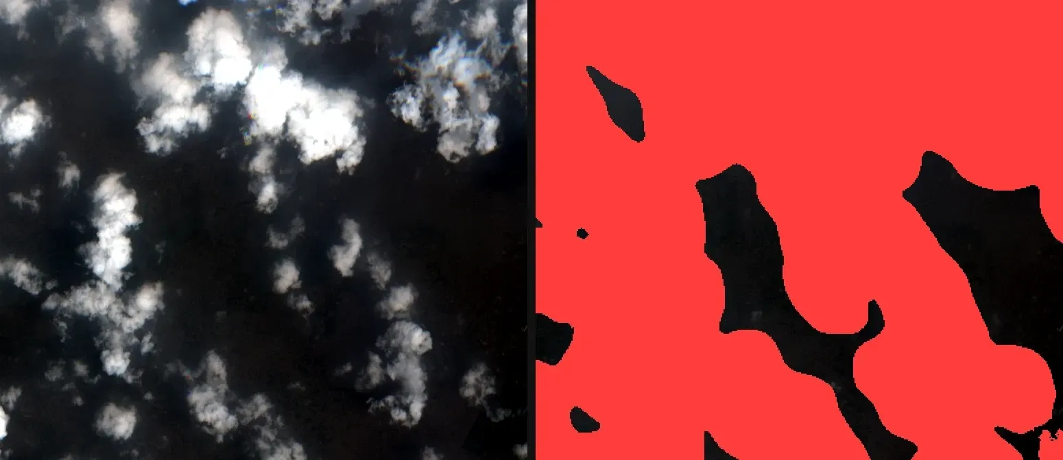
FIG. 02 Punjab, 15 July 2024: true colour (left) and the SCL cloud mask over the area (right). Contains modified Copernicus Sentinel data 2024.
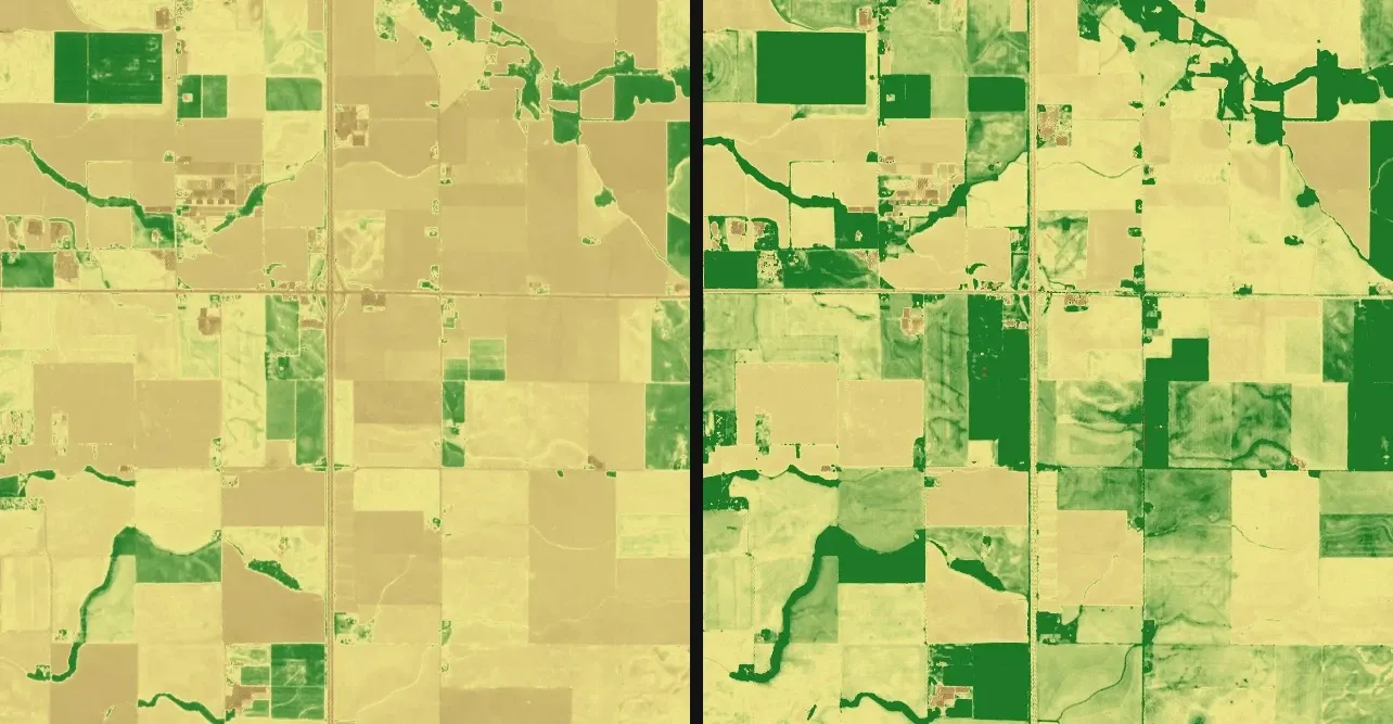
FIG. 03 Willamette Valley, 2 August 2024: NDVI without the reflectance offset (left, mean 0.299) and with it (right, mean 0.497). Contains modified Copernicus Sentinel data 2024.